It is a somewhat advanced tutorial, so if you have not already done so, it might be a good idea to work through the Introductory Tutorial first.
A huge number of examples are, of course, available on the CD that comes with the book. The difference is that there the programs come without explanation. If you would like to work with the diagrams as you read this teacher's tutorial, all of them can be found in the subdirectory Reference/Teachers of the installation directory (which is where Geometer's browser should point automatically).
Warning: A lot of internet browsers will have trouble with some of the special mathematics characters used here, such as the one for the angle symbol, for Greek letters, et cetera. So if you see some text with mysterious rectangles instead of characters, your browser can't draw the characters, and you'll either have to guess what they are, or look at the more formal documentation with Acrobat of PostScript files.
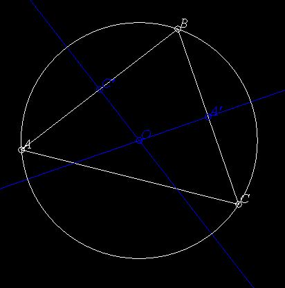
Let's warm up with a simple construction—we'll construct the circumcircle of an arbitrary triangle.

The first thing to do is to get a (fairly) firm idea in your head about how you want the finished Geometer diagram to behave. In this example, I've chosen to do it as a five step process (see the figure above):
If you're not doing it already, run Geometer on your computer and follow along as we construct this example.
Here is how I would do it in detail.
.geometry "version 0.31";
v1 = .free(-0.407186, 0.0209581, "A");
v2 = .free(0.239521, 0.598802, "B");
v3 = .free(0.502994, -0.161677, "C");
l1 = .l.vv(v1, v2);
l2 = .l.vv(v2, v3);
l3 = .l.vv(v3, v1);
v4 = .v.vvmid(v1, v2, "C'");
v5 = .v.vvmid(v2, v3, "A'");
l4 = .l.vlperp(v4, l1, .longline);
l5 = .l.vlperp(v5, l2, .longline);
v6 = .v.ll(l4, l5, "O");
c1 = .c.vv(v6, v1);
Most of what appears above is pretty obvious: v1, v2, and v3 are the points labeled A, B, and C, l1 is the line connecting v1 and v2 (or, in other words, the line AB), and similarly for lines l2 and l3.
Look at the rest of the entries to make sure you understand how they correspond to the items in your drawing. They appear in exactly the same order you issued the GUI commands, and if you have any doubt, the Advanced Reference Guide.
v4 = .v.vvmid(v1, v2, "C'");
to become:
v4 = .v.vvmid(v1, v2, "C'", [.in, .blink, .blue]);
The information between the square brackets is the color information. The .in says that on layer 0, the color is invisible. Then the .blink says to paint this point in a blinking color on layer 1, and the final .blue says that from layer 2 on, the object should always be painted in blue. Remember the comma after the text: "C'".
After you make this edit, save the file using the Save command under the File pull-down menu in the text editor window. If you did make a typing error, type the OK button on the alert menu and you will be put back in the text editor with the line containing the error highlighted. If you made no error, you should be back to the GUI form of Geometer, but the point C' will be invisible.
Notice that all the rest of your diagram is visible in all steps. That's because by default, all items are created to appear on all layers.
.l0;
(That's "ell-zero", not "ell-oh"). It tells Geometer to begin displaying this diagram displaying only layer zero.
Save your changes (use Save under the Edit pulldown, or simply by typing Ctrl-s), and note that the diagram appears with only the "0" layer lit under Layer Control. If you like, you can press the Next button a few times to see that it still has the desired behavior for the appearance of point C'.
.geometry "version 0.31";
.l0;
v1 = .free(-0.407186, 0.0209581, "A");
v2 = .free(0.239521, 0.598802, "B");
v3 = .free(0.502994, -0.161677, "C");
l1 = .l.vv(v1, v2);
l2 = .l.vv(v2, v3);
l3 = .l.vv(v3, v1);
v4 = .v.vvmid(v1, v2, [.in, .blink, .blue], "C'");
v5 = .v.vvmid(v2, v3, "A'");
l4 = .l.vlperp(v4, l1, .longline);
l5 = .l.vlperp(v5, l2, .longline);
v6 = .v.ll(l4, l5, "O");
c1 = .c.vv(v6, v1);
Notice that Geometer has changed what you put in! The .l0; command has been moved to the top of the file, and the layer information you typed in for point C' has been moved to appear before the "C'".
The reason is that slight reorderings like this make no difference, and Geometer doesn't remember exactly what you typed in—it just remembers the effect you want, so when it prints its version, that version may be slightly different from what you typed. The layer command moved to a different line, but the vast majority of other reorderings are within a single line.
 l3 =
.l.vv(v3, v1);X
and save the file with Ctrl-S. Geometer will barf and will display an alert notifier with the obscure message, "Line 9: Expected '='{}". For now ignore the message and press the OK button on the notifier and you will be returned to the text editor with line 9 highlighted. Usually all that's required is a quick glance to see what's wrong and to fix it, in this case by deleting the X you just typed. Go ahead and delete the X and save the file again, and you should be back to where you were.
Now edit the file again, but add an X to the ends of two different lines and try to save the file. You'll get an error message, but only about the first error, and only that line will be highlighted. Fix that error, try to save again, and you'll be pointed at the second bad line, et cetera. Geometer basically gives up as soon as it hits the first error.
Note that sometimes the error is really on the previous line—Geometer may not notice there's anything wrong until it tries to interpret the next line.
With more experience, you can use the information in the error message as well. The one above, "Line 9: Expected '='{}", occurred because beginning with the X, Geometer was expecting something like
X = .free(0, 0);
Geometer does not require the commands to be one per line; there can be multiple commands on a single line, or one command can stretch across many input lines.
.geometry "version 0.31";
.l0;
v1 = .free(-0.407186, 0.0209581, "A");
v2 = .free(0.239521, 0.598802, "B");
v3 = .free(0.502994, -0.161677, "C");
l1 = .l.vv(v1, v2);
l2 = .l.vv(v2, v3);
l3 = .l.vv(v3, v1);
v4 = .v.vvmid(v1, v2, [.in, .blink, .blue], "C'");
v5 = .v.vvmid(v2, v3, "A'");
l4 = .l.vlperp(v4, l1, .longline);
l5 = .l.vlperp(v5, l2, .longline);
v6 = .v.ll(l4, l5, "O");
c1 = .c.vv(v6, v1);
.geometry "version 0.31";
.l0;
v1 = .free(-0.407186, 0.0209581, "A");
v2 = .free(0.239521, 0.598802, "B");
v3 = .free(0.502994, -0.161677, "C");
l1 = .l.vv(v1, v2);
l2 = .l.vv(v2, v3);
l3 = .l.vv(v3, v1);
v4 = .v.vvmid(v1, v2, [.in, .blink, .blue], "C'");
v5 = .v.vvmid(v2, v3, [.in, .blink, .blue], "A'");
l4 = .l.vlperp(v4, l1, [2 .in, .blink, .blue], .longline);
l5 = .l.vlperp(v5, l2, [2 .in, .blink, .blue], .longline);
v6 = .v.ll(l4, l5, [3 .in, .blink, .blue], "O");
c1 = .c.vv(v6, v1, [4 .in, .blink, .white]);
After you have completed the edits above, test your diagram by pressing the Next button to see that it behaves correctly---on layer 0, only the triangle appears. On layer 1, the two midpoints, A' and C' appear blinking. On layer 2, the perpendicular bisectors appear blinking, and the midpoints change to blue. On layer 3, point O appears, blinking, and the perpendicular bisectors are blue. On layer 4, the required circle is blinking---all the other construction items are blue. On layers 5 and beyond, the circle is white.
The only new thing that we've done is to add some multipliers in the color/layer specifications. In the specification for point O, for example:
v6 = .v.ll(l4, l5, [3 .in, .blink, .blue], "O");
the 3 in front of the .in signifies that three invisible layers appear. This multiplier could appear anywhere in the specification, and you don't need to use it on input. For example, suppose you wanted some item to be red for the first three steps, then invisible for 2, and finally to appear white for the rest of the layers, you could type this color/layer specification that will work fine:
[.red, .red, .red, .in, .in, .white]
But after you save it, Geometer will print it as:
[3 .red, 2 .in, .white]
.geometry "version 0.31";
.l0;
v1 = .free(-0.437126, 0.0748503, "A");
v2 = .free(0.239521, 0.598802, "B");
v3 = .free(0.502994, -0.161677, "C");
l1 = .l.vv(v1, v2);
l2 = .l.vv(v2, v3);
l3 = .l.vv(v3, v1);
v4 = .v.vvmid(v1, v2, [.in, .blink, .blue], "C'");
v5 = .v.vvmid(v2, v3, [.in, .blink, .blue], "A'");
l4 = .l.vlperp(v4, l1, [2 .in, .blink, .blue], .longline);
l5 = .l.vlperp(v5, l2, [2 .in, .blink, .blue], .longline);
v6 = .v.ll(l4, l5, [3 .in, .blink, .blue], "O");
c1 = .c.vv(v6, v1, [.white, 3 .in, .blink, .white]);
.text("Given \triangleABC, construct its circumcircle.", .l0);
.text("Move points A, B, and C to see
what 'circumcircle' means.", .yellow, .l0);
.text("Find the midpoints C' and A' of
segments AB and BC, respectively.", .l1);
.text("Construct a line through C' perpendicular
to AB and a line through A' perpendicular
to BC.", .l2);
.text("Let O be the intersection of those
perpendicular bisectors.", .l3);
.text("The circle centered at O that passes
through A is the required circumcircle.", .l4);
.text("Press 'Next' to continue ...", .red, .tol3);
A lot of new ideas are used above---we'll look at them command by command.
In the first line you typed:
.text("Given \triangleABC, construct its circumcircle.", .l0);
the text that appears between the double quotes will appear in the Geometer diagram. Geometer understands certain combinations of letters, like "\triangle", above, to represent a special symbol, in this case, the triangle symbol: Δ. The line will appear in Geometer as:
Given ΔABC, construct its circumcircle.
The line will appear in the default color (white), and the final token on the line, ".l0", tells Geometer to display it only on layer 0. In this case, ".l0" is shorthand for: "[.white, .in]".
The next two lines:
.text("Move points A, B, and C to see
what 'circumcircle' means.", .yellow, .l0);
Display the two lines of text between the double quotes as two lines in Geometer. The lines will also appear in layer 0 only, but this set will be in yellow. The text will look like this on the screen (in yellow, of course):
Move points A, B, and C to see
what 'circumcircle' means.
Notice that the line breaks on the screen appear whereever newlines were typed in the .text command.
Not much new appears in the next four commands, except that the text is presented on different layers: .l1 for layer 1, et cetera.
Finally, the last line:
.text("Press 'Next' to continue ...", .red, .tol3);
is drawn in red, and the layer control ".tol3" means that it appears from layer 0 to layer 3---in other words, on four layers. It could have been done with: [4 .red, .in].
Geometer always interprets a file in order, so if there are multiple lines of text that appear on the visible layer, they will be drawn as they appear in the file. In the example above, there are three .text commands that display something on layer 0, so the layer 0 text will look like this on the Geometer screen:
Given ΔABC, construct its circumcircle.
Move points A, B, and C to see
what 'circumcircle' means.
Press 'Next' to continue ...
The first line will be drawn in white, the next two in yellow, and the final line in red.
There, you've finished with the first example! One final thing worth noting is that although the demonstration "officially" ends on the fifth layer (layer 4), if you step on to layer 5, you get a non-blinking version of everything that is suitable for printing. In addition, the printing version has no text (although it could, if you wanted to, but usually the text in your document will be sufficient). The figure above is what you get if you "print" the figure that appears on layer 5.
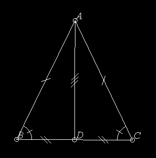
The first problem we face is how to construct the diagram so that the student will be able to manipulate it in such a way that two of the lines will remain the same length. We are trying to construct something like Figure XXX, where segments AB and AC are always equal. There are various approaches, but for this example, I've chosen to make points B and C completely free, but to constrain point A to lie on the perpendicular bisector of the segment BC.
Here are the steps I followed; as before, I highly recommend that you follow along and generate the same diagram in your own version of Geometer.
In fact, the fastest approach is this: Double-click on Free P so that you can create a bunch of points, click once to make the point A, and immediately type Ctrl-d to delete it, then click twice more to make points labelled B and C. Finally, click Cancel Repeat Mode to get out of the repeat creation mode.
Test your diagram (and save it to disk if you like) by moving points A, B, and C. B and C should move completely freely, but point A should be constrained to lie on the perpendicular bisector of BC (and hence the lengths of AB and AC will remain equal, as we desired).
To complete the proof, we are going to need line segment AD, so draw that now as well.
Let's begin by marking the lines and angles that are supposed to be congruent so that the student can see more clearly what's going on. Select line segment AB and use the cascaded pull-down Style menu to set that line to 1 Slash. Do the same thing for segment AC. Both will now be drawn with a single slash through them.
We also want to show that the base angles, ∠ACB and ∠ABC are equal, so first use the Angle Type button in the control panel to set the default angle type to 1 Slash. Now use the PPP=>A command in the control panel to make two angles above. Click on the points in the order they appear in the angle description; for example, to draw ∠ACB, click on point A, then C, and finally, B. In certain cases, the angles you get may be "inside-out"---in other words, the reflex angle is drawn. If that happens, there's a Flip Angle command under the Edit pull-down menu that's also available as the keyboard Ctrl-a command.
.geometry "version 0.31";
v2 = .free(-0.254936, -0.168969, "B");
v3 = .free(0.429834, -0.171934, "C");
l1 = .l.vv(v2, v3);
v1 = .v.vvmid(v2, v3, "D");
l2 = .l.vlperp(v1, l1, .in);
v4 = .vonl(l2, 0.090513, 0.537185, "A");
l3 = .l.vv(v4, v2, .line1slash);
l4 = .l.vv(v4, v3, .line1slash);
l5 = .l.vv(v4, v1);
ang1 = .a.vvv(v4, v3, v2, .slash1);
ang2 = .a.vvv(v3, v2, v4, .slash1);
Convert it to what follows by adding the layer color information to four of the lines, and by adding the .text entries:
.geometry "version 0.31";
.l0;
v2 = .free(-0.254936, -0.168969, "B");
v3 = .free(0.429834, -0.171934, "C");
l1 = .l.vv(v2, v3);
v1 = .v.vvmid(v2, v3, [.in, .blink, .blue], "D");
l2 = .l.vlperp(v1, l1, .in);
v4 = .vonl(l2, 0.090513, 0.537185, "A");
l3 = .l.vv(v4, v2, .line1slash);
l4 = .l.vv(v4, v3, .line1slash);
l5 = .l.vv(v4, v1, [2 .in, .blink, .blue]);
ang1 = .a.vvv(v4, v3, v2, [.white, 3 .in, .blink, .white], .slash1);
ang2 = .a.vvv(v3, v2, v4, [.white, 3 .in, .blink, .white], .slash1);
.text("Show that if AB \congruent AC in \triangleABC, then
\angleACB = \angleABC.", .l0);
.text("Move points A, B, and C.", .yellow, .l0);
.text("Let D be the midpoint of segment BC, so
BD \congruent CD.", .l1);
.text("Construct line AD which is congruent
to itself.", .l2);
.text("\triangleACD \congruent \triangleABD by SSS, since
AB \congruent AC, AD \congruent AD, and BD \congruent CD.", .l3);
.text("Since \triangleACD \congruent \triangleABD, we
have \angleACB \congruent \angleABC, which we
wanted to show.", .l4);
.text("Press 'Next' to continue ...", .red, .tol3);
You now have a proof that is acceptable, but which can be vastly improved.
For example, it would be nice to have all the congruent segments marked as are AB and AC, and it would be nice to somehow highlight the two triangles that we showed to be congruent: ΔACD and ΔABD.
The easiest way to do this is using the GUI of Geometer. We want the segments BD and CD to be congruent, so just use the PP=>L command to add those lines, but before you do that, issue the 2 Slash command under the Styles→Lines cascading pull-down menu. The layer colors will be wrong, but we can fix those later in the text editor.
Using Next, we can also get to a point where we can see the segment AD, and put three slashes on it with the 3 Slash command under the same cascading menu.
To fix the layer colors for the segments BD and CD, use the editor to convert:
l6 = .l.vv(v2, v1, .l1, .line2slash);
l7 = .l.vv(v3, v1, .l1, .line2slash);
to
l6 = .l.vv(v2, v1, [.in, .white], .line2slash);
l7 = .l.vv(v3, v1, [.in, .white], .line2slash);
Save these changes, and test the file again---it's a little better, but we can improve it just a little by having all three sets of congruent sides blinking in three different blinking colors (.blink, .blink1, and .blink2) on layer 3, where we state that the triangles are congruent by SSS. Those modifications, plus a couple of others to make everything appear in white on the layer past the end yield a file that looks something like this:
.geometry "version 0.31";
.l0;
v2 = .free(-0.254936, -0.168969, "B");
v3 = .free(0.429834, -0.171934, "C");
l1 = .l.vv(v2, v3);
v1 = .v.vvmid(v2, v3, [.in, .blink, 2 .blue, .white], "D");
l2 = .l.vlperp(v1, l1, .in);
v4 = .vonl(l2, 0.090513, 0.537185, "A");
l3 = .l.vv(v4, v2, [3 .white, .blink, .white], .line1slash);
l4 = .l.vv(v4, v3, [3 .white, .blink, .white], .line1slash);
l5 = .l.vv(v4, v1, [2 .in, .blink, .blink2, .white], .line3slash);
ang1 = .a.vvv(v4, v3, v2, [.white, 3 .in, .blink, .white], .slash1);
ang2 = .a.vvv(v3, v2, v4, [.white, 3 .in, .blink, .white], .slash1);
.text("Show that if AB \congruent AC in \triangleABC, then
\angleACB = \angleABC.", .l0);
.text("Move points A, B, and C.", .yellow, .l0);
.text("Let D be the midpoint of segment BC, so
BD \congruent CD.", .l1);
.text("Construct line AD which is congruent
to itself.", .l2);
.text("\triangleACD \congruent \triangleABD by SSS, since
AB \congruent AC, AD \congruent AD, and BD \congruent CD.", .l3);
.text("Since \triangleACD \congruent \triangleABD, we
have \angleACB \congruent \angleABC, which we
wanted to show.", .l4);
.text("Press 'Next' to continue ...", .red, .tol3);
l6 = .l.vv(v2, v1, [.in, 2 .white, .blink1, .white], .line2slash);
l7 = .l.vv(v3, v1, [.in, 2 .white, .blink1, .white], .line2slash);
Next, we'll construct a proof that the diagonals of a trapezoid are perpendicular. (A trapezoid is a convex quadrilateral with four equal sides.)
The first problem is to draw a figure that the student can manipulate in such a way that four points always form a trapezoid. The solution I selected has two completely free points, A and B, and the third point C lies on a circle centered at B and passing through A. This will guarantee that AB ≅ BC. To do this construction, put down two free points A and B, draw the circle centered at B and passing through A, and then use the P on C to make the point C lying on that circle. We don't want the circle cluttering up the diagram, so click on the circle to select it, and paint it the invisible color.
The locations of A, B, and C completely determine D. Since we know that the theorem is true, we can take advantage of it, and construct D. The easiest way I could think to do it is to draw the line AC (which we will need later as part of the proof), and then to reflect the point B across AC to get the fourth point D of the trapezoid. To do this, you need the command LP=>P Mirror that can be found in the cascading pulldown menu Primitives→Point.
Connect the four points AB, BC, CD, and DA with segments to form the trapezoid. Now kick yourself, select the segments individually, and convert each to a segment with a single slash going through it with the cascading pull-down menu Styles→Line→1 Slash. (Kick yourself because if you had selected this style before drawing the four lines, they would all automatically have gotten the slash.)
Finally, draw in the two diagonals (but this time, remember to turn off the slash before doing so with the menu entry Styles→Line→No Mark).
Test the diagram by moving points A, B, and C to make sure that D moves appropriately, save the file, and now you're ready to start building in the proof.
Use the editor to put in the first few lines that explain the theorem to prove, and remember to add the line .l0; to put Geometer into the proof mode when the file is loaded. In short, add these lines. (Note the use of the \congruent and \perp commands that draw the congruence symbol (≅), and the perpendicular symbol (⊥).
.l0;
.text("Prove that the diagonals of a trapezoid
are perpendicular.  In other words, if
AB \congruent BC \congruent CD \congruent DA then AC \perp BD.
Move points A, B, and C.", .l0);
Next we'll show that various internal angles are equal (for example, ∠ACD ≅ ∠CAD) since they lie opposite equal sides. To do this, make the angles appear at the appropriate steps of the proof, and at the same time, it would be nice if the sides opposite them also blinked, perhaps in a different color.
We continue to step through the proof, adding a line of text at a time, and then modifying the layer colors of the various lines and angles so that things blink and stop blinking at the correct times, and eventually, we get to the following fairly good proof:
.geometry "version 0.31";
.l0;
v1 = .free(-0.299401, 0.508982, "A");
v2 = .free(-0.38024, -0.11976, "B");
c1 = .c.vv(v2, v1, .in);
v3 = .vonc(c1, 0.22768, 0.0599201, "C");
l1 = .l.vv(v1, v3, [3 .white, .blink2, .white]);
v6 = .v.lvmirror(l1, v2, "D");
l2 = .l.vv(v1, v2, [2 .white, .blink1, .blink, 3 .white,
    .blink2, .white], .line1slash);
l3 = .l.vv(v2, v3, [2 .white, 2 .blink1, .white, .blink,
    .white, .blink2, .white], .line1slash);
l4 = .l.vv(v3, v6, [.white, .blink1, .white, .blink1,
    .white], .line1slash);
l5 = .l.vv(v6, v1, [.white, .blink1, .white, .blink,
    .white, .blink, .white], .line1slash);
l6 = .l.vv(v2, v6);
v7 = .v.ll(l1, l6, .l7on, "O");
.text("Prove that the diagonals of a trapezoid
are perpendicular.  In other words, if
AB \congruent BC \congruent CD \congruent DA then AC \perp BD.
Move points A, B, and C.", .l0);
.text("In \triangleACD, AD \congruent CD, so
\angle CAD \congruent \angle ACD.", .l1);
ang1 = .a.vvv(v7, v1, v6, [.in, .blink, 2 .white,
    .blink, .white], .slash1);
ang2 = .a.vvv(v6, v3, v1, [.in, .blink, 2 .white, .blink,
    .white], .slash1);
.text("Similarly, n \triangleACB, AB \congruent CB, so
\angle CAB \congruent \angle BCA.", .l2);
ang3 = .a.vvv(v2, v1, v7, [2 .in, .blink, .white, .in], .slash2);
ang4 = .a.vvv(v1, v3, v2, [2 .in, .blink, .white, .in], .slash2);
.text("But AD \congruent AB, CD \congruent CB, and AC
is congruent to itself, so \triangleBAC \congruent \triangleDAC.", .l3);
.text("Since \triangleBAC \congruent \triangleDAC, we have
\angleDAC \congruent \angleDCA \congruent \angleBAC \congruent \angleBCA.",
    .l4);
ang5 = .a.vvv(v1, v3, v2, [4 .in, .blink, 2 .white, .blink,
    .white], .slash1);
ang6 = .a.vvv(v2, v1, v3, [4 .in, .blink, 2 .white, .blink,
    .white], .slash1);
.text("Since \angleBCA \congruent \angleDAC, lines
AD and BC are parallel, so the transveral
BD makes \angleADB \congruent CBD.", .l5);
ang7 = .a.vvv(v1, v6, v2, [5 .in, 2 .blink1, .white], .ring2);
ang8 = .a.vvv(v3, v2, v6, [5 .in, 3 .blink1, .white], .ring2);
.text("But since AB \congruent AD in \triangle ABD
we have \angle DBA \congruent ADB \congruent \angleCBD.", .l6);
ang9 = .a.vvv(v6, v2, v1, [6 .in, 2 .blink1, .white], .ring2);
.text("Let O be the intersection of AC and DB.  Then
since AB \congruent BC, \angleOBA \congruent \angleOBC, and
\angleBAO \congruent \angleBCO, \triangleAOB \congruent \triangleCOB.",
    .l7);
.text("Since \triangleAOB \congruent \triangleCOB,
\angleBOA \congruent \angleBOC, but since those
are supplementary angles,
\angleBOA = \angle BOC = 90\degrees.", .l8);
ang10 = .a.vvv(v1, v7, v2, [8 .in, .blink, .white], .right);
ang11 = .a.vvv(v2, v7, v3, [8 .in, .blink, .white], .right);
.text("Press 'Next' to continue ...", .red, .tol7);
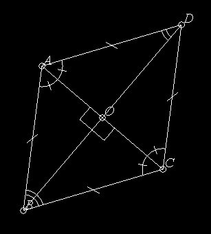
Try loading a copy of this proof from the file Trapezoid.T and step through it as you read the following comments about what goes on for each layer setting.
The code above was not modified to its current condition in one pass. I stepped to each stage of the proof, figured out what colors I wanted to change, and then went in with the editor and changed the layer colors on those items for that step only. Then I tested the entire diagram again. It took about an hour to get it to its current state, starting from scratch.
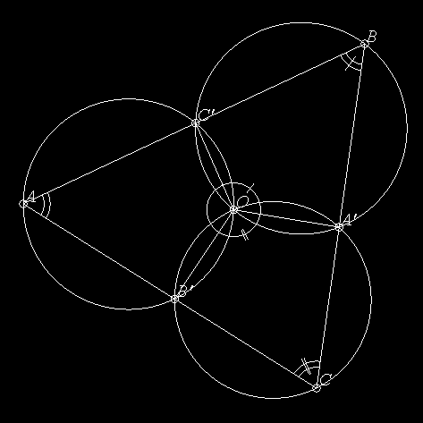
If points A', B', and C' are selected on the sides BC, CA, and AB of ΔABC, then the three circles passing through AB'C', through BA'C', and through CB'A' all meet at a point.
This is an easy construction to make using Geometer, and the code for the diagram ThreeCircles.T is shown below:
.geometry "version 0.31";
.l0;
v1 = .free(-0.571856, 0.0598802, "A");
v2 = .free(0.571856, 0.595808, "B");
v3 = .free(0.41018, -0.556886, "C");
l1 = .l.vv(v1, v2);
l2 = .l.vv(v2, v3);
l3 = .l.vv(v3, v1);
v4 = .vonl(l1, 0.005177, 0.33027, "C'");
v5 = .vonl(l2, 0.48574, -0.0181719, "A'");
v6 = .vonl(l3, -0.0652644, -0.258284, "B'");
c1 = .c.vvv(v6, v5, v3);
c2 = .c.vvv(v5, v4, v2);
c3 = .c.vvv(v1, v4, v6, [.white, 3 .in, .magenta, .white]);
v7 = .v.cc(c1, c2, 2, [.in, .blink, .white], "O");
.text("Theorem: Given any \triangleABC, select
points A', B', and C' on BC, CA, and AB,
respectively.  The circles passing through
CB'A', BA'C', and AC'B' all meet at a point.
Move points A, B, C, A', B', and C'.", .l0);
.text("Let O be the intersection different from
A' of circles BA'C' and CB'A'.  Construct segments
OA', OB' and OC'.", .l1);
l4 = .l.vv(v7, v5, [.in, .blink, .white]);
l5 = .l.vv(v7, v6, [.in, .blink, .white]);
l6 = .l.vv(v7, v4, [.in, .blink, .white]);
.text("Since CA'OB' and BA'OC' are concyclic,
we have:", .l2);
.text("(1) \angle A'OC' + \angle C'BA' = 180\degrees
(2) \angle B'OA' + \angle A'CB' = 180\degrees", [2 .in, .white, .yellow, .in]);
ang1 = .a.vvv(v5, v7, v4, [2 .in, .blink, .blink1, .white], .slash1);
ang2 = .a.vvv(v4, v2, v5, [2 .in, 2 .blink, .white], .slash2);
ang3 = .a.vvv(v6, v7, v5, [2 .in, 2 .blink1, .white], .dslash1);
ang4 = .a.vvv(v5, v3, v6, [2 .in, .blink1, .blink, .white], .dslash2);
ang5 = .a.vvv(v4, v7, v6, [3 .in, .blink1, .white]);
ang6 = .a.vvv(v3, v1, v2, [3 .in, .blink, .white], .ring2);
.text("(3) \angleC'BA' + \angleA'CB' + \angleB'AC' = 180\degrees
(4) \angleA'OC' + \angleB'OA' + \angle C'OB' = 360\degrees
Calculate (3)+(4)-(1)-(2) giving", .l3);
.text("Since", .l4);
.text("\angleC'OB' + \angle B'AC' = 180\degrees", .l3, .l4);
.text("We know that AC'OB' are concyclic.", .l4);
.text("Press 'Next' to continue ...", .red, .tol3);
Step through the proof in Geometer as you read the discussion about each layer below, and refer to the text above to see how the various effects are achieved.
This example provides a nice example of how the various layer colors work. The goal is to illustrate a binary counter where the digit 0 is represented by the color red and the digit 1 by the color green. As you step through the "proof", one layer at a time is shown, and the colors of four different squres will display the binary value for that number as a combination of red and green squares.
You can make the squares (or whatever other shapes you may like) using Geometer's GUI, or, as I did in this example, you can simply type in the exact coordintes that you like so that the objects are uniform and uniformly spaced. Here is the code for the binary counter:
.geometry "version 0.31";
.l0;
v1a = .pinned(0.5, -0.1, .in);
v1b = .pinned(0.5, 0.1, .in);
v1c = .pinned(0.7, 0.1, .in);
v1d = .pinned(0.7, -0.1, .in);
v2a = .pinned(0.2, -0.1, .in);
v2b = .pinned(0.2, 0.1, .in);
v2c = .pinned(0.4, 0.1, .in);
v2d = .pinned(0.4, -0.1, .in);
v4a = .pinned(-0.1, -0.1, .in);
v4b = .pinned(-0.1, 0.1, .in);
v4c = .pinned(0.1, 0.1, .in);
v4d = .pinned(0.1, -0.1, .in);
v8a = .pinned(-0.4, -0.1, .in);
v8b = .pinned(-0.4, 0.1, .in);
v8c = .pinned(-0.2, 0.1, .in);
v8d = .pinned(-0.2, -0.1, .in);
p1 = .polygon(4, v1a, v1b, v1c, v1d, [.red, .green, .red, .green,
          .red, .green, .red, .green, .red, .green, .red, .green,
          .red, .green, .red, .green], .solidpoly);
p2 = .polygon(4, v2a, v2b, v2c, v2d, [2 .red, 2 .green, 2 .red,
          2 .green, 2 .red, 2 .green, 2 .red, .green], .solidpoly);
p4 = .polygon(4, v4a, v4b, v4c, v4d, [4 .red, 4 .green, 4 .red,
          .green], .solidpoly);
p8 = .polygon(4, v8a, v8b, v8c, v8d, [8 .red, .green], .solidpoly);
The four polygons, p1, p2, p4, and p8, represent the four binary digits. The one's digit alternates red and green on every step; the two's digit alternates every two steps, et cetera.
The code below improves on the counter above. Instead of using red and green to represent the digits, we actually draw out a zero and a one. The zero is made with an ellipse, and the one with a line segment. To draw the zero, I played around with the five points until I had a shape I liked; then I pinned the points by converting the .free to .pinned in the editor. To get exact copies of my ellipses, I simply translated the original points to the right to make additional copies.
Then I used the same alternation of colors in the layer color commands, but made sure that when the zero was showing, the one was not, and vice-versa.
Here's the code:
.geometry "version 0.31";
.l0;
va = .pinned(0, 0.01, .in);
vb = .pinned(0.05, 0, .in);
vc = .pinned(0.026, 0.2, .in);
vd = .pinned(0.025, -0.2, .in);
ve = .pinned(0.0479042, -0.0898204, .in);
wa = .pinned(0.025, 0.2, .in);
wb = .pinned(0.025, -0.2, .in);
va1 = .v.vtranslate(va, 0.100000, 0.000000, .in);
vb1 = .v.vtranslate(vb, 0.100000, 0.000000, .in);
vc1 = .v.vtranslate(vc, 0.100000, 0.000000, .in);
vd1 = .v.vtranslate(vd, 0.100000, 0.000000, .in);
ve1 = .v.vtranslate(ve, 0.100000, 0.000000, .in);
wa1 = .v.vtranslate(wa, 0.100000, 0.000000, .in);
wb1 = .v.vtranslate(wb, 0.100000, 0.000000, .in);
va2 = .v.vtranslate(va, 0.200000, 0.000000, .in);
vb2 = .v.vtranslate(vb, 0.200000, 0.000000, .in);
vc2 = .v.vtranslate(vc, 0.200000, 0.000000, .in);
vd2 = .v.vtranslate(vd, 0.200000, 0.000000, .in);
ve2 = .v.vtranslate(ve, 0.200000, 0.000000, .in);
wa2 = .v.vtranslate(wa, 0.200000, 0.000000, .in);
wb2 = .v.vtranslate(wb, 0.200000, 0.000000, .in);
va3 = .v.vtranslate(va, 0.300000, 0.000000, .in);
vb3 = .v.vtranslate(vb, 0.300000, 0.000000, .in);
vc3 = .v.vtranslate(vc, 0.300000, 0.000000, .in);
vd3 = .v.vtranslate(vd, 0.300000, 0.000000, .in);
ve3 = .v.vtranslate(ve, 0.300000, 0.000000, .in);
wa3 = .v.vtranslate(wa, 0.300000, 0.000000, .in);
wb3 = .v.vtranslate(wb, 0.300000, 0.000000, .in);
zero1 = .conic.vvvvv(va3, vb3, vc3, vd3, ve3, [.white, .in,
      .white, .in, .white, .in, .white, .in, .white, .in,
      .white, .in, .white, .in, .white, .in]);
zero2 = .conic.vvvvv(va2, vb2, vc2, vd2, ve2, [2 .white,
       2 .in, 2 .white, 2 .in, 2 .white, 2 .in, 2 .white, .in]);
zero4 = .conic.vvvvv(va1, vb1, vc1, vd1, ve1, [4 .white,
       4 .in, 4 .white, .in]);
zero8 = .conic.vvvvv(va, vb, vc, vd, ve, [8 .white, .in]);
one1 = .l.vv(wa3, wb3, [.in, .white, .in, .white, .in, .white,
       .in, .white, .in, .white, .in, .white, .in, .white,
       .in, .white]);
one2 = .l.vv(wa2, wb2, [2 .in, 2 .white, 2 .in, 2 .white,
       2 .in, 2 .white, 2 .in, .white]);
one4 = .l.vv(wa1, wb1, [4 .in, 4 .white, 4 .in, .white]);
one8 = .l.vv(wa, wb, [8 .in, .white]);
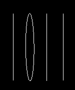
The figure above shows the result that appears on layer number 11.
You can (mis)use Geometer as a general graphing package, although it can be a bit clumsy. A lot of the clumsiness comes from the fact that Geometer insists on a coordiante system with (0,0) in the center of the drawing area and that runs from -1.0 to 1.0 in the shorter screen direction. In what follows, we'll assume that the Geometer drawing area is square, so its coordinate system will run from -1.0 to 1.0 in both directions.
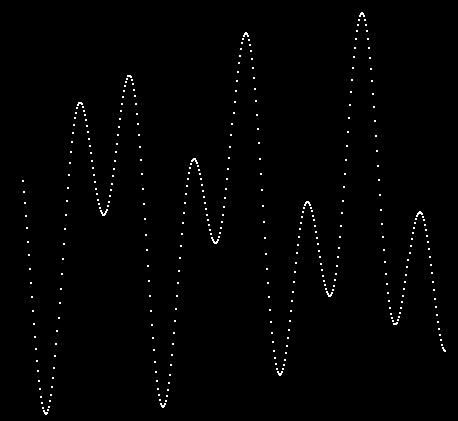
For this example, we'll simply plot the function:
f(x) = cos 5x + sin 11x.
Just eyeballing the function above, we can see that it must range in size between -2.0 and 2.0, so we'll probably want to multiply the x and y values by a number slightly smaller than 0.5 to make it fit. Thus, the input (x) values will also range from -2.0 to 2.0. In fact, if we make this input range a bit larger, the curve will run off both ends, and will thus be guaranteed to fill as much of the screen as possible. (By the way, the angles are measured in radians, or we wont see much!)
Once we've made those decisions, the code is pretty simple:
.geometry "version 0.31";
.radianmode;
x = .script(-2.100000, 2.100000, 0.010000);
y = .f.rpn(x, 5.000000, .mul, .cos, x,
        11.000000, .mul, .sin, .add, 0.450000,
        .mul);
x1 = .f.rpn(x, 0.450000, .mul);
v = .v.ff(x1, y, .smear, .dot);
The first line .radianmode; puts Geometer in radianmode; it measures angles in degrees by default.
The second line tells Geometer that the diagram is to be a script---that the Run Script button should be active, and when pressed, Geometer will repeatedly evaluate the entire program using values of x that run between -2.1 and 2.1 in steps of 0.01. If the spacing of the dots is wrong, you can make them more or less dense by changing value of 0.01 appropriately.
The third line does the calculation of the y-value: it takes x, multiplies it by 5 and takes the cosine, then takes another copy of x and multiplies it by 11, takes the sine, and then adds together the values. Finally, the result is multiplied by 0.45 (a number slightly less than 0.5) to keep the plot in range. x1 is a similarly scaled value of x.
Finally, a point v is plotted with coordinates x1 and y. It is plotted in the smearing color so that all the dots will appear on the screen. It is drawn as a single dot (using .dot as point type) so as not to clutter the screen too much.
The final result can be seen in Figure \ref{fig:plot}.
It is also easy to plot parametric curves in the same way, where both the x- and y-coordinates are functions of a parameter t. Just let the .script command generate values of t, calculate x and y values using .f.rpn, and plot away.
Functions in polar coordinates are slightly more interesting. In this case, the function relates the angle θ with the radius, ρ. ρ or θ can usually be the parameter, and the other variable is calculated in terms of it, but then the resulting values must be converted to x- and y-coordinates so Geometer can deal with them. The conversion is simple, however:
x = ρcosθ
y = ρsinθ.
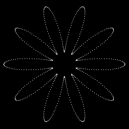
As an example, let's plot the function
ρ = 0.5 + (cos 10θ)/3.
The result can be seen in the figure above.
Here's the code to do it:
.geometry "version 0.31"; .radianmode; theta = .script(0.000000, 6.283100, 0.010000); rho = .f.rpn(0.500000, theta, 10.000000, .mul, .cos,3.000000, .div, .add); x = .f.rpn(theta, .cos, rho, .mul); y = .f.rpn(theta, .sin, rho, .mul); v = .v.ff(x, y, .smear, .dot);
An ellipse is commonly defined in terms of two foci F_1 and F_2 and a length, l. The ellipse is the set of all points P such that F_1P + F_2P = l. Equivalently, it can be defined in terms of the foci F_1, F_2, and a point P, and the point X is on the ellipse if F_1P + F_2P = F_1X + F_2X. This second definition is better for Geometer diagrams since Geometer allows you to manipulate points freely, and it's a little messier to manipulate a length. The conic sections that can be defined in Geometer, however, only include those that pass through 5 points, or those that are tangent to 5 lines.
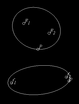
In this section we'll construct a macro that takes the two foci and a point on the boundary as input and draws the ellipse. In the figure above is a demonstration of two calls to the macro, one with focus points at F_1, F_2, and passing through point P, and the other with foci f_1, f_2, and passing through p.
Here is the Geometer code to generate the figure above:
.geometry "version 0.32";
v1 = .free(-0.0299401, 0.479042, "F\sub{1}");
v2 = .free(0.389222, 0.317365, "F\sub{2}");
v3 = .free(0.203593, 0.0508982, "P");
v4 = .free(-0.233533, -0.505988, "f\sub{1}");
v5 = .free(0.673653, -0.41018, "f\sub{2}");
v6 = .free(0.718563, -0.473054, "p");
.macro conic(.vertex f1, .vertex f2, .vertex p)
{
    d1 = .f.vv(f1, p);
    d2 = .f.vv(f2, p);
    sum = .f.rpn(d1, d2, .add);
    r1 = .f.rpn(sum, 0.550000, .mul);
    r2 = .f.rpn(sum, 0.450000, .mul);
    c1 = .c.vf(f1, r1, .in);
    c2 = .c.vf(f2, r1, .in);
    c3 = .c.vf(f1, r2, .in);
    c4 = .c.vf(f2, r2, .in);
    v4 = .v.cc(c2, c3, 1, .in, "D");
    v5 = .v.cc(c1, c4, 2, .in, "E");
    v6 = .v.cc(c1, c4, 1, .in, "F");
    v7 = .v.cc(c2, c3, 2, .in, "G");
    con1 = .conic.vvvvv(p, v7, v6, v5, v4);
}
conic(v1, v2, v3);
conic(v4, v5, v6);
The code is fairly straight-forward---it takes the sample points, calculates the length (called sum), and then draws a pair of circles around the points of lengths .45 and .55 of the total length. The intersections of these circles will be points on the ellipse as well as the original point. The ellipse is the conic that passes through the original point and through the four circle intersections.
This example isn't particularly useful but it does make use of a bunch of new diagram construction techniques, especially the use of the arithmetic operations available for floating point numbers as well as some other tricks.
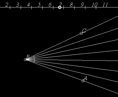
The diagram will consist of a fixed line marked from 2 to 11 at the top of the screen, and an angle ∠ABC below whose size can be modified. The user can drag a point along the line at the top of the screen and it's position will represent an integer n from 2 to 11. The angle below is divided into two n equal parts. In other words, if n=2, the angle is bisected; if n=3, it is trisected, and so on. The figure above shows the diagram when the slider is in the region corresponding to n=7. The angle ∠ABC is divided into seven equal parts.
The code to do this was basically all typed in by hand. For the discussion below, it is broken into various chunks, but in the Geometer file it all appears together.
.geometry "version 0.31";
v1 = .v.ff(-1.000000, 0.800000, .in);
v2 = .v.ff(1.000000, 0.800000, .in);
l1 = .l.vv(v1, v2, .longline);
vp2 = .pinned(-0.9, 0.8, .nomark, "2");
vp3 = .pinned(-0.7, 0.8, .nomark, "3");
vp4 = .pinned(-0.5, 0.8, .nomark, "4");
vp5 = .pinned(-0.3, 0.8, .nomark, "5");
vp6 = .pinned(-0.1, 0.8, .nomark, "6");
vp7 = .pinned(0.1, 0.8, .nomark, "7");
vp8 = .pinned(0.3, 0.8, .nomark, "8");
vp9 = .pinned(0.5, 0.8, .nomark, "9");
vp10 = .pinned(0.7, 0.8, .nomark, "10");
vp11 = .pinned(0.9, 0.8, .nomark, "11");
vm1 = .pinned(-0.8, 0.8, .plus);
vm2 = .pinned(-0.6, 0.8, .plus);
vm3 = .pinned(-0.4, 0.8, .plus);
vm4 = .pinned(-0.2, 0.8, .plus);
vm5 = .pinned(0, 0.8, .plus);
vm6 = .pinned(0.2, 0.8, .plus);
vm7 = .pinned(0.4, 0.8, .plus);
vm8 = .pinned(0.6, 0.8, .plus);
vm9 = .pinned(0.8, 0.8, .plus);
tab = .vonl(l1, -0.140719, 0.8, .cyan);
All this first chunk of code does is to draw the rule at the top of the viewing area. The coordinates for a square viewing area run from -1.0 to 1.0 in both directions, so the rule runs all the way across the drawing area with a y-coordinate of 0.8. The vm1, vm2, ... points are marked with crosses so that they divide the rule into 11 roughly equally-sized pieces and the vp2, vp3, ... points show no mark, but they appear between the other points and label the regions on the rule. Finally, the point called tab is stuck on the rule and can slide back and forth on it.
Note that all the points are pinned. This is so you can't inadvertantly move them, but so that they will show up in the drawing.
value = .f.vxcoord(tab);
count = .f.rpn(value, 1.000000, .add, 0.200000, .div,
        2.000000, .add, .truncate);
The two lines above determine the value of n (which is called count in the code here). The first line takes the x-coordinate of the point tab that can slide along the line and stores it in a floating point number called value.
The next line converts value to a number between 2 and 11. We know that originally value is between -1.0 and 1.0 so if we add 1.0 to it and divide that result by 0.2 we will obtain a number between 0 and 10 (and it will, in fact be less than 10---something like 9.999 is the maximum value it can have).
Add 2 to that and truncate to the nearest integer and we've got a number between (and including) 2 and 11.
The .f.rpn line above does exactly the calculation described above. It puts value on the stack, then it puts 1.0 on the stack and adds the two, leaving the single result value+1 on the stack.
The next two entries, 0.200000 and .div, divide the number on the stack by 0.2. The next two entries add 2 to the result, and the final .truncate command rounds down to the nearest integer, so the result stored in count will be an integer between 2 and 11.
v3 = .free(0.55988, -0.571856, "A");
v4 = .free(-0.51497, -0.176647, "B");
v5 = .free(0.526946, 0.314371, "C");
l2 = .l.vv(v4, v3, .ray12);
l3 = .l.vv(v4, v5, .ray12);
ang = .a.vvv(v3, v4, v5);
The lines above were the only ones in this example that were entered using the GUI of Geometer. They draw the angle that is to be subdivided in the middle of the screen.
m2 = .f.rpn(ang, count, .div);
This line takes the measure of angle ang, divides it by count, and stores the result in the variable m2. The main angle has to be broken into a bunch of angles all having equal measures m2.
The problem, of course, is that depending on the size of count a different number of those angles need to be drawn. Geometer is not very good at conditional code, so what can be done?
x1 = .f.rpn(m2, 1.000000, count, .mod, .mul);
x2 = .f.rpn(m2, 2.000000, count, .mod, .mul);
x3 = .f.rpn(m2, 3.000000, count, .mod, .mul);
x4 = .f.rpn(m2, 4.000000, count, .mod, .mul);
x5 = .f.rpn(m2, 5.000000, count, .mod, .mul);
x6 = .f.rpn(m2, 6.000000, count, .mod, .mul);
x7 = .f.rpn(m2, 7.000000, count, .mod, .mul);
x8 = .f.rpn(m2, 8.000000, count, .mod, .mul);
x9 = .f.rpn(m2, 9.000000, count, .mod, .mul);
x10 = .f.rpn(m2, 10.000000, count, .mod, .mul);
OK, here's the dirty trick---we're going to draw 11 dividing lines, no matter what the angle is. It's just that for small values of count, lots of them will be drawn on top of each other.
Basically, to find the angle size, we take m2 and multiply it by ten values: 1 (mod count), 2 (mod count), ..., 10 (mod count). Let's look at the situation where count=4 to see what's going on:
0 = 4 (mod 4) = 8 (mod 4)
1 = 1 (mod 4) = 5 (mod 4) = 9 (mod 4)
2 = 2 (mod 4) = 6 (mod 4) = 10 (mod 4)
3 = 3 (mod 4) = 7 (mod 4),
so ten lines are drawn, but two of them are drawn 3 times and two of them are drawn twice.
But now we have the angles, so all that remains is to draw them. The following straightforward code does the trick. It could probably be made shorter with a macro, but it was pretty simple just to get one set of three lines working correctly, and then to make nine more copies which were modified in the obvious way:
ang1 = .a.f(x1);
vsplit1 = .v.avv(ang1, v3, v4, .in);
lsplit = .l.vv(v4, vsplit1, .ray12);
ang2 = .a.f(x2);
vsplit2 = .v.avv(ang2, v3, v4, .in);
lsplit2 = .l.vv(v4, vsplit2, .ray12);
ang3 = .a.f(x3);
vsplit3 = .v.avv(ang3, v3, v4, .in);
lsplit3 = .l.vv(v4, vsplit3, .ray12);
ang4 = .a.f(x4);
vsplit4 = .v.avv(ang4, v3, v4, .in);
lsplit4 = .l.vv(v4, vsplit4, .ray12);
ang5 = .a.f(x5);
vsplit5 = .v.avv(ang5, v3, v4, .in);
lsplit5 = .l.vv(v4, vsplit5, .ray12);
ang6 = .a.f(x6);
vsplit6 = .v.avv(ang6, v3, v4, .in);
lsplit6 = .l.vv(v4, vsplit6, .ray12);
ang7 = .a.f(x7);
vsplit7 = .v.avv(ang7, v3, v4, .in);
lsplit7 = .l.vv(v4, vsplit7, .ray12);
ang8 = .a.f(x8);
vsplit8 = .v.avv(ang8, v3, v4, .in);
lsplit8 = .l.vv(v4, vsplit8, .ray12);
ang9 = .a.f(x9);
vsplit9 = .v.avv(ang9, v3, v4, .in);
lsplit9 = .l.vv(v4, vsplit9, .ray12);
ang10 = .a.f(x10);
vsplit10 = .v.avv(ang10, v3, v4, .in);
lsplit10 = .l.vv(v4, vsplit10, .ray12);
The 30 lines above can be replaced by the following 16 lines if you're willing to use a macro. Ten more of the earlier lines can also be moved into the macro if you wish---the lines where x1, ..., x10 were defined.
.macro newangle(.flt f)
{
    ang1 = .a.f(f);
    vsplit1 = .v.avv(ang1, v3, v4, .in);
    lsplit1 = .l.vv(v4, vsplit1, .ray12);
}
newangle(x1);
newangle(x2);
newangle(x3);
newangle(x4);
newangle(x5);
newangle(x6);
newangle(x7);
newangle(x8);
newangle(x9);
newangle(x10);
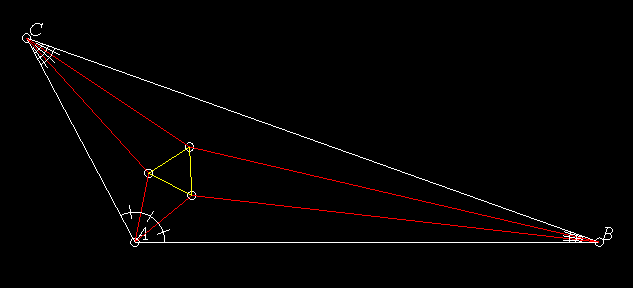
Morley's Theorem (see the figure above) states that if you examine the intersections of the angle trisectors of any triangle, they will meet in pairs to form an equilateral triangle.
Here's the actual Geometer code to draw the basic diagram for Morley's Theorem. The key parts are the three sets of five lines beginning with the .a.vvv commands. This gets the angle from the three points. That angle is then divided by 3 (well, multiplied by 1/3, and the resulting number is converted back to an angle. That new angle is then used to construct two more points on the trisectors. There is some funny stuff to make the picture pretty---a lot of the lines are invisible because they were used in the construction, but in the nice illustration only parts of them are shown. Much of the diagram below can be constructed by pointing and clicking, but you will need to type in the three sections of code that generate the sets of trisectors.
.geometry "version 0.2";
v1 = .free(-0.874251, -0.760479, "A");
v2 = .free(0.0658683, 0.766467, "C");
v3 = .free(0.811377, -0.601796, "B");
l1 = .l.vv(v1, v2);
l2 = .l.vv(v2, v3);
l3 = .l.vv(v3, v1);
a = .a.vvv(v1, v2, v3, .noangle);
ll2 = .f.rpn(a, 0.333333, .mul);
a3 = .a.f(ll2);
vv1 = .v.avv(a3, v1, v2, .in);
ww1 = .v.avv(a3, vv1, v2, .in);
l4 = .l.vv(v2, ww1, .in, .ray12);
l5 = .l.vv(v2, vv1, .in, .ray12);
b = .a.vvv(v2, v3, v1, .noangle);
ll4 = .f.rpn(b, 0.333333, .mul);
b3 = .a.f(ll4);
vv2 = .v.avv(b3, v2, v3, .in);
ww2 = .v.avv(b3, vv2, v3, .in);
l6 = .l.vv(v3, ww2, .in, .ray12);
l7 = .l.vv(v3, vv2, .in, .ray12);
c = .a.vvv(v3, v1, v2, .noangle);
ll6 = .f.rpn(c, 0.333333, .mul);
c3 = .a.f(ll6);
vv3 = .v.avv(c3, v3, v1, .in);
ww3 = .v.avv(c3, vv3, v1, .in);
l8 = .l.vv(v1, ww3, .in, .ray12);
l9 = .l.vv(v1, vv3, .in, .ray12);
v4 = .v.ll(l8, l5, "Y");
v5 = .v.ll(l6, l9, "Z");
v6 = .v.ll(l7, l4, "X");
l10 = .l.vv(v1, v5, .red);
l11 = .l.vv(v1, v4, .red);
l12 = .l.vv(v4, v2, .red);
l13 = .l.vv(v2, v6, .red);
l14 = .l.vv(v6, v3, .red);
l15 = .l.vv(v3, v5, .red);
l16 = .l.vv(v5, v6, .yellow);
l17 = .l.vv(v6, v4, .yellow);
l18 = .l.vv(v4, v5, .yellow);
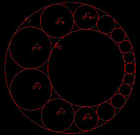
How can the figure above be constructed using a computer geometry program?
Obviously, a set of equally-spaced circles that exactly fill the ring between two concentric circles was constructed, and the result was inverted to obtain a Steiner Porism with a lopsided pair of enclosing rings. The inverted circles will exactly fill the space between the lopsided rings.
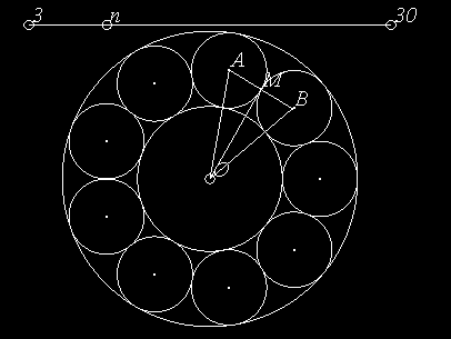
It is not hard to work out the relative sizes of a pair of concentric circles that will allow for some fixed number n of circles to fit between them. In the figure above we see what we need to begin. In this case, there are nine circles, but let's just call that number n. The central angle between any pair of circle centers is 360°/n, so vertex angle ∠AOB = 360° of the isosceles triangle in the figure.
If that figure, ΔOMA is a right triangle where M is the point of tangency of two adjacent circles. Suppose the radius of the inner circle is R_1 and the radius of the small surrounding circles is R_2 (which will make the radius of the larger circle R_1 + 2R_2).
Then
sin(180°/n) = R_2/(R_1 + R_2))
and we can solve for R_2:
R_2 = R_1 sin(180°/n)/(1 - sin(180°/n)).
The Geometer code below draws the figure (and a lot more besides). It includes a sort of slider at the top to change the number of surrounding circles to be anything from 3 to 30. The point labelled n can slide between the pinned v1 and v2. The ratio is then converted using the .f.rpn commands to a number n between 3 and 30. Then r2 is calculated using the formula we obtained in the previous paragraph. (r1 is arbitrarily set to be .4.)
Next, a macro is defined to draw circle number i. It finds the sine and cosine of the angle 180°(i/n) and multiplies them by the offset from the center, R_1 + R_2. These are the coordinates for the center circle number i, and a circle of radius r2 is drawn around that center.
Then 30 circles are drawn. The fact that fewer than 30 are needed doesn't matter; if i is too big, the circle corresponding to i will be drawn exactly on top of a previous one.
Note that since all the calculations are done in absolute coordinates, the circles will all be centered at the origin of the drawing, in the exact middle of the drawing area. This could be done differently, if desired. The final few lines of code draw the circles that inscribe and circumscribe that ring of circles. These, of course, also need to be calculated using the .f.rpn commands.
Finally, the listing is condensed from what Geometer would really put into its file---it would put each of the macro calls to circ on a separate line. By condensing them, you're saved looking at a page of almost identical commands.
This code, of course, only draws the circles between a pair of concentric circles. Additional code is needed to draw the Steiner Porism, since each of these circles should be inverted (which can be done most conveniently inside the macro). Then all the circles but the inverted versions should be painted the invisible color so all that appears in the Geometer diagram is the porism.
.geometry "version 0.2";
// Listing condensed by hand --
// all the calls to the circ macro were on different lines.
r1 = .f.rpn(0.400000);
v1 = .pinned(-1, 0.9, "3");
v2 = .pinned(1, 0.9, "30");
l1 = .l.vv(v1, v2);
v3 = .vonl(l1, -0.569395, 0.9, "n");
rat = .f.vvvratio(v1, v3, v2);
n = .f.rpn(rat, 27.500000, .mul, 3.500000, .add,
        .truncate);
a = .f.rpn(180.000000, n, .div);
r2 = .f.rpn(a, .sin, .dup, 1.000000, .exch,
        .sub, .exch, r1, .mul, .exch,
        .div);
.macro circ(.flt i)
{
    x = .f.rpn(a, 2.000000, .mul, i, .mul,
        .cos, r1, r2, .add, .mul);
    y = .f.rpn(a, 2.000000, .mul, i, .mul,
        .sin, r1, r2, .add, .mul);
    v = .v.ff(x, y, .dot);
    c = .c.vf(v, r2);
}
circ(0.000000); circ(1.000000); circ(2.000000);
circ(3.000000); circ(4.000000); circ(5.000000);
circ(6.000000); circ(7.000000); circ(8.000000);
circ(9.000000); circ(10.000000); circ(11.000000);
circ(12.000000); circ(13.000000); circ(14.000000);
circ(15.000000); circ(16.000000); circ(17.000000);
circ(18.000000); circ(19.000000); circ(20.000000);
circ(21.000000); circ(22.000000); circ(23.000000);
circ(24.000000); circ(25.000000); circ(26.000000);
circ(27.000000); circ(28.000000); circ(29.000000);
orig = .pinned(0, 0);
cin = .c.vf(orig, r1);
rout = .f.rpn(r1, r2, 2.000000, .mul, .add);
cout = .c.vf(orig, rout);
Apollonius' problem is to find three circles tangent to a given circle. This is done with a series of inversions, and is a bit tricky to illustrate with a Geometer diagram.
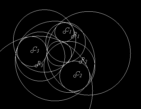
There are up to eight possible solutions, and in the figure above an example is shown where all eight mutually tangent circles are shown.
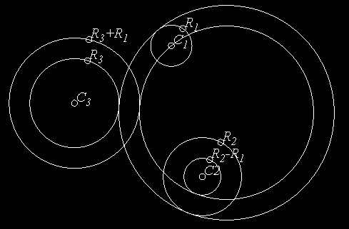
The key idea is this: If we choose the circle of smallest radius and shrink it to a point, and at the same time either add or subtract the radius of the smallest circle to or from the radii of the larger circles, then solving Apollonius' problem for a point and two circles will yield a circle whose radius can be increased or decreased by the radius of the smallest circle to yield a solution. (There are direct solutions as well that involve moving the line or lines parallel to themselves by a distance equal to the diameter of the smallest circle, just as we expand and shrink the diameters of the larger circles in the three-circle solution.)
The figure above demonstrates the general idea. The original circles for which the problem is to be solved are centered at C_1, C_2, and C_3, and they have radii R_1, R_2, and R_3, respectively. Assume that R_1 is the smallest of the three radii. One solution can be obtained by drawing a circle centered at C_2 of radius R_2-R_1 and by drawing a circle about C_3 of radius R_3+R_1. Using techniques we learned earlier in the chapter, we can find a circle that is tangent to those new circles with the modified radii and passing through C_1 as shown in the figure. If that circle's radius is then increased by R_1, we have one of the eight possible solutions to the problem of finding circles mutually tangent to the three given circles.
Beware: This is trickier than it seems. Remember that there are up to four solutions to the "two circles and a point" problem, possibly having tangencies on both sides of both circles. Only one of these four circles can have its radius increased and still be tangent to the original circles. In fact, if you play with the {Geometer} diagram that generates the figure showing the solution for Apollonius' problem, you'll find that it works only for a limited range of values around the initial configuration---increase or decrease the radii too much and you'll find that the solutions jump to the other sides of circles, and on expansion or contraction of those circles, they no longer solve the problem.
It took a lot of work to produce this {Geometer} diagram---the editor was used repeatedly. Clearly, it could have been done with standard construction techniques, but the solution would have been hundreds of lines long. What follows is the complete code for that diagram, but broken into chunks with some commentary following each chunk.
It is pretty clear from the names which lines were done using the mouse and which were drawn with the editor. The mouse interface always makes up the same sorts of names, like v1, v2, et cetera, for points, and c1, c2, ..., for circles. Names like r2sub were typed in the editor. Also, there are a huge number of items drawn in the "invisible" color (.in). Typically, they were drawn in a color-coded way (internal tangents one color, external in another, for example), and when they were no longer needed for the construction, they were "erased" by turning them to an invisible color.
.geometry "version 0.2";
v1 = .free(0.169341, 0.542551, "C\sub{1}");
v2 = .free(0.348837, 0.44186, "R\sub{1}");
v3 = .free(0.392748, -0.401592, "C\sub{2}");
v4 = .free(0.51497, -0.101796, "R\sub{2}");
v5 = .free(-0.526167, 0.12827, "C\sub{3}");
v6 = .free(-0.436047, -0.180233, "R\sub{3}");
c1 = .c.vv(v5, v6);
c2 = .c.vv(v1, v2);
c3 = .c.vv(v3, v4);
r1 = .f.vv(v1, v2);
r2 = .f.vv(v3, v4);
r3 = .f.vv(v5, v6);
r2sub = .f.rpn(r2, r1, .sub);
r3sub = .f.rpn(r3, r1, .sub);
r2add = .f.rpn(r1, r2, .add);
r3add = .f.rpn(r3, r1, .add);
c3sub = .c.vf(v5, r3sub, .in);
c2sub = .c.vf(v3, r2sub, .in);
c3add = .c.vf(v5, r3add, .in);
c2add = .c.vf(v3, r2add, .in);
The code above draws the three initial circles, and it assumes that the radius r1 is the smallest of the three radii. r1 is added and subtracted from each of the other two radii and four circles are constructed centered at the same places as the other two circles, but with radii increased or decreased the appropriate amount.
v7 = .free(0.365897, 1.00522, .in, "7");
c4 = .c.vv(v1, v7, .in);
c5 = .c.ccinv(c2add, c4, .in);
c6 = .c.ccinv(c3add, c4, .in);
l2 = .l.ccext(c6, c5, 2, .in, .longline);
l3 = .l.ccext(c6, c5, 1, .in, .longline);
c7 = .c.ccinv(c3sub, c4, .in);
c8 = .c.ccinv(c2sub, c4, .in);
l21 = .l.ccext(c7, c8, 2, .in, .longline);
l31 = .l.ccext(c7, c8, 1, .in, .longline);
l1 = .l.ccint(c7, c5, 2, .in);
l4 = .l.ccint(c7, c5, 1, .in);
l5 = .l.ccint(c8, c6, 1, .in);
l6 = .l.ccint(c6, c8, 2, .in);
An arbitrary circle of inversion c4 is drawn, and all four of the circles with modified radii are inverted in it. The common external and internal tangents to various pairs of those four circles are also drawn (after inversion, the center of the smallest circle went to infinity, so inverted solution to Apollonius' problem for two circles and a point will be these four lines tangent to the inverses of the circles with modified radii).
c10 = .c.lcinv(l2, c4, .in);
c11 = .c.lcinv(l3, c4, .in);
c14 = .c.lcinv(l21, c4, .in);
c15 = .c.lcinv(l31, c4, .in);
c9 = .c.lcinv(l1, c4, .in);
c12 = .c.lcinv(l6, c4, .in);
c13 = .c.lcinv(l4, c4, .in);
c16 = .c.lcinv(l5, c4, .in);
The tangent lines are inverted to find solution circles going through the center of C_1 and tangent to the circles with modified radii.
v8 = .v.ccenter(c9, .in, "I");
v9 = .v.ccenter(c12, .in, "J");
v10 = .v.ccenter(c13, .in, "K");
v11 = .v.ccenter(c16, .in, "L");
v12 = .vonc(c9, -0.474808, -0.263661, .in, "M");
v13 = .vonc(c12, 0.0527364, -0.175382, .in, "N");
v14 = .vonc(c13, -0.103302, -0.0870917, .in, "O");
v15 = .vonc(c16, 0.0408249, -0.602817, .in, "P");
rad1 = .f.vv(v8, v12);
rad11 = .f.rpn(rad1, r1, .sub);
cf1 = .c.vf(v8, rad11);
rad2 = .f.vv(v9, v13);
rad22 = .f.rpn(rad2, r1, .add);
cf2 = .c.vf(v9, rad22);
rad3 = .f.vv(v10, v14);
rad33 = .f.rpn(rad3, r1, .add);
cf3 = .c.vf(v10, rad33);
rad4 = .f.vv(v11, v15);
rad44 = .f.rpn(rad4, r1, .sub);
cf4 = .c.vf(v11, rad44);
The centers and points on the radii of four of the circles are found. From these, the radii can be determined, and r1 can be added or subtracted as appropriate, and the new final circles can be found.
v16 = .v.ccenter(c11, .in, "Q");
v17 = .v.ccenter(c15, .in, "R");
v18 = .v.ccenter(c14, .in, "S");
v19 = .v.ccenter(c10, .in, "T");
v20 = .vonc(c11, -0.00771487, 0.608311, .in, "U");
v21 = .vonc(c15, -0.347598, 0.492195, .in, "V");
v22 = .vonc(c14, -0.314278, 0.371898, .in, "W");
v23 = .vonc(c10, 0.261844, 0.534324, .in, "X");
rad5 = .f.vv(v16, v20);
rad55 = .f.rpn(rad5, r1, .sub);
cf5 = .c.vf(v16, rad55);
rad6 = .f.vv(v17, v21);
rad66 = .f.rpn(rad6, r1, .add);
cf6 = .c.vf(v17, rad66);
rad7 = .f.vv(v18, v22);
rad77 = .f.rpn(rad7, r1, .sub);
cf7 = .c.vf(v18, rad77);
rad8 = .f.vv(v19, v23);
rad88 = .f.rpn(rad8, r1, .add);
cf8 = .c.vf(v19, rad88);
The operation above is repeated on the final set of four circles.

If we use the solution to Apollonius' problem in the previous section to obtain the circumscribing circle, we are faced with the problem that the construction there required the knowledge of which of the circles was the smallest. Not only that, but if there are 8 possible circles tangent to the three excircles, which one is the one that circumscribes them?
Feuerbach's Theorem comes to our aid, however. Feuerbach's Theorem states that the nine-point circle of a triangle is tangent to the three excircles of the triangle (and to the incircle as well, but that doesn't matter to us here).
If we can find an inversion that takes the excircles into themselves, the nine-point circle will be inverted to be the required tangent circle. Circles are inverted to themselves by any circle that is orthogonal to them. The circle orthogonal to all three excircles has its center at the radical center of the three circles, and we can find its radius by drawing a tangent to any of the circles from the radical center and using that point of tangency as a point on the diameter of the required circle.
So how do we find the radical center? It is the intersection of any pair or radical axes of pairs of the circles. The radical axis is easy to construct if the two circles intersect, but in this case, we know that none of the pairs do. So the usual trick is to find a circle that passes through both circles, to find the radical center of those three (the two non-intersecting circles and the one that intersects them both), and that point will lie on the radical axis. Then choose another circle that intersects both and find the radical center for those three. That will be another point on the radical axis of the two non-intersecting circles. With two points on the radical axis, we can construct it.
There are a couple of strategies for finding a circle that intersects pairs of circles. Perhaps the easiest would be to find a circle that passes through their centers and through any other point, but then we'd need two pairs of such circles. This will work fine, but the solution here is to find two circles that intersect all three of the excircles so they can be used to find both of the radical axes. One circle that's guaranteed to work is the one that passes through the three circle centers. Another is obtained by taking the nine-point circle and making it a tiny bit larger so that it intersects all three. Remember that it is tangent to the three, so making it a tiny bit larger will cause it to intersect the three. In the construction here, it is 10% larger.
Once we have the circle orthogonal to all three circles, invert the nine-point circle through it, and it is the required outer tangent circle.
But now we need to find those points of tangency, and using the circle-circle intersection method is risky---due to numerical round-off, the circles might miss by a millionth of an inch and there will be no intersection. The easiest thing to do is to connect the centers of the circles with lines (which will pass through both circles perpendicularly), and find the intersections of those lines with the circles.
Here is the code that does the construction interleaved with a discussion of how it works. The vast majority was constructed with the Geometer GUI, but obviously a text editor was used from time to time.
It may be easier to follow this with the Geometer diagram displayed on the screen. If the meaning of any of the invisible points doesn't make sense, open the diagram with the text editor, change the invisible point to some obvious color, and redisplay.
.geometry "version 0.40";
v1 = .free(-0.158683, 0.0718563, "A");
v2 = .free(0.00299401, 0.374251, "B");
v3 = .free(0.149701, 0.122754, "C");
l1 = .l.vv(v1, v2, .longline);
l2 = .l.vv(v2, v3, .longline);
l3 = .l.vv(v3, v1, .longline);
c2 = .c.lll(l1, l2, l3, 2);
c3 = .c.lll(l2, l1, l3, 2);
c4 = .c.lll(l1, l3, l2, 2);
v27 = .v.ccenter(c3, .in);
v28 = .v.ccenter(c2, .in);
v29 = .v.ccenter(c4, .in);
The code above makes the triangle, draws the three excircles, and finds their centers. The centers are needed to make one of the circles that passes through all three of the excircles.
v4 = .v.vvmid(v1, v2, .in);
v5 = .v.vvmid(v2, v3, .in);
v6 = .v.vvmid(v3, v1, .in);
c5 = .c.vvv(v4, v5, v6, .in);
v9 = .v.ccenter(c5, .in);
r = .f.vv(v9, v6);
r1 = .f.rpn(r, 1.100000, .mul);
c6 = .c.vf(v9, r1, .in);
c7 = .c.vvv(v27, v28, v29, .in);
Circle c5 is the nine-point circle (we know that the nine-point circle passes through the three midpoints of the sides). Then r is the radius of the nine-point circle, and we multiply it by $1.1$ to get a new radius for a slightly larger circle centered at the same point (v9, the center of the nine-point circle), but guaranteed to intersect all three. c6 is that larger circle, and c7 is the circle passing through the centers of all three excircles.
v7 = .v.cc(c7, c2, 2, .in);
v8 = .v.cc(c7, c2, 1, .in);
v10 = .v.cc(c3, c7, 2, .in);
v11 = .v.cc(c3, c7, 1, .in);
v12 = .v.cc(c2, c6, 1, .in);
v13 = .v.cc(c2, c6, 2, .in);
v14 = .v.cc(c3, c6, 2, .in);
v15 = .v.cc(c3, c6, 1, .in);
Here are the eight intersections of the circles passing through all three excircles with the excircles themselves.
l4 = .l.vv(v11, v10, .in, .longline);
l5 = .l.vv(v7, v8, .in, .longline);
v16 = .v.ll(l4, l5, .in);
l6 = .l.vv(v14, v15, .in, .longline);
l7 = .l.vv(v13, v12, .in, .longline);
v17 = .v.ll(l6, l7, .in);
l8 = .l.vv(v16, v17, .in, .longline);
v18 = .v.cc(c4, c7, 2, .in);
v19 = .v.cc(c4, c7, 1, .in);
v20 = .v.cc(c4, c6, 1, .in);
v21 = .v.cc(c4, c6, 2, .in);
l9 = .l.vv(v21, v20, .in, .longline);
v22 = .v.ll(l9, l7, .in);
l10 = .l.vv(v18, v19, .in, .longline);
v23 = .v.ll(l5, l10, .in);
l11 = .l.vv(v22, v23, .in, .longline);
v24 = .v.ll(l11, l8, .in);
This is the construction of the radical center. Two pairs of radical axes are made for each of two pairs of excircles, their intersections are found to get two points on the radical axis of each pair of excircles, and then the radical axes are intersected at v24 which is the radical center of the three excircles.
l12 = .l.vc(v24, c2, 2, .in, .longline);
v25 = .v.lc(l12, c2, 2, .in);
c1 = .c.vv(v24, v25, .in);
c8 = .c.ccinv(c5, c1);
v25 is the point of tangency of a line from the radical center to one of the excircles. c1 is the circle of inversion, and c8 is the inverted nine-point circle that is the exterior tangent of the three excircles.
v26 = .v.ccenter(c8, .in);
l13 = .l.vv(v26, v29, .in, .longline);
l14 = .l.vv(v26, v28, .in, .longline);
l15 = .l.vv(v26, v27, .in, .longline);
v30 = .v.lc(l15, c8, 2);
v31 = .v.lc(l14, c8, 2);
v32 = .v.lc(l13, c8, 2);
Finally, the centers of the excircles and the center of the surrounding circle are connected with lines that are intersected with the various circles to get the exterior points.
l16 = .l.vv(v2, v32);
l17 = .l.vv(v1, v31);
l18 = .l.vv(v3, v30);
v33 = .v.ll(l16, l17, "P");
.text("Apollonius Point:  If the points of tangency
of the three excircles and their circumscribed
circle are connected to the opposite vertices of
a triangle, those lines are concurrent at
Apollonius' Point.", .l0);
Those exterior points are connected to the vertices of the triangle, and the point of Apollonius is found. There's also a short chunk of text to describe the construction.